A peek inside LookupJoin

I won't be describing in the details the internals of LookupJoin. They seem a bit too big and complicated. Partially it's because the code is of an older origin, and not using the newer shortcuts. Partially it's because when I wrote it, I've tried to optimize by translating the rows to an array format instead of referring to the fields by names, and that made the code more tricky. Partially, the code has grown more complex due to all the added options. And partially the functionality just is a little tricky by itself.

But, for debugging purposes, the LookupJoin constructor can return the auto-generated code of the joiner function. It's done with the option "saveJoinerTo":

  saveJoinerTo => \$code,

This snippet will cause the auto-generated code to be placed into the variable $code. This provides a glimpse into the internal workings of the joiner.

This is the joiner code from the first example:

sub # ($inLabel, $rowop, $self)
{
  my ($inLabel, $rowop, $self) = @_;
  #print STDERR "DEBUGX LookupJoin " . $self->{name} . " in: ", $rowop->printP(), "\n";

  my $opcode = $rowop->getOpcode(); # pass the opcode
  my $row = $rowop->getRow();

  my @leftdata = $row->toArray();

  my $resRowType = $self->{resultRowType};
  my $resLabel = $self->{outputLabel};

  my $lookuprow = $self->{rightRowType}->makeRowHash(
    source => $leftdata[1],
    external => $leftdata[2],
    );
  
  #print STDERR "DEBUGX " . $self->{name} . " lookup: ", $lookuprow->printP(), "\n";
  my $rh = $self->{rightTable}->findIdx($self->{rightIdxType}, $lookuprow);
  Carp::confess("$!") unless defined $rh;

  my @rightdata; # fields from the right side, defaults to all-undef, if no data found
  my @result; # the result rows will be collected here

  if (!$rh->isNull()) {
    #print STDERR "DEBUGX " . $self->{name} . " found data: " . $rh->getRow()->printP() . "\n";
    @rightdata = $rh->getRow()->toArray();
  }

    my @resdata = ($leftdata[0],
    $leftdata[1],
    $leftdata[2],
    $leftdata[3],
    $rightdata[2],
    );
    my $resrowop = $resLabel->makeRowop($opcode, $resRowType->makeRowArray(@resdata));
    #print STDERR "DEBUGX " . $self->{name} . " +out: ", $resrowop->printP(), "\n";
    Carp::confess("$!") unless defined $resrowop;
    Carp::confess("$!") 
      unless $resLabel->getUnit()->call($resrowop);
    
}

This is the joiner code from the example with the manual iteration:

sub  # ($self, $row)
{
  my ($self, $row) = @_;

  #print STDERR "DEBUGX LookupJoin " . $self->{name} . " in: ", $row->printP(), "\n";

  my @leftdata = $row->toArray();

  my $lookuprow = $self->{rightRowType}->makeRowHash(
    source => $leftdata[1],
    external => $leftdata[2],
    );
  
  #print STDERR "DEBUGX " . $self->{name} . " lookup: ", $lookuprow->printP(), "\n";
  my $rh = $self->{rightTable}->findIdx($self->{rightIdxType}, $lookuprow);
  Carp::confess("$!") unless defined $rh;

  my @rightdata; # fields from the right side, defaults to all-undef, if no data found
  my @result; # the result rows will be collected here

  if (!$rh->isNull()) {
    #print STDERR "DEBUGX " . $self->{name} . " found data: " . $rh->getRow()->printP() . "\n";
    @rightdata = $rh->getRow()->toArray();
  }

    my @resdata = ($leftdata[0],
    $leftdata[1],
    $leftdata[2],
    $leftdata[3],
    $rightdata[2],
    );
    push @result, $self->{resultRowType}->makeRowArray(@resdata);
    #print STDERR "DEBUGX " . $self->{name} . " +out: ", $result[$#result]->printP(), "\n";
  return @result;
}

It takes different arguments because now it's not an input label handler but a common function that gets called from both the label handler and the lookup() method. And it collects the rows in an array to be returned instead of immediately passing them on.

This is the joiner code from the example with multiple rows matching on the right side:

sub # ($inLabel, $rowop, $self)
{
  my ($inLabel, $rowop, $self) = @_;
  #print STDERR "DEBUGX LookupJoin " . $self->{name} . " in: ", $rowop->printP(), "\n";

  my $opcode = $rowop->getOpcode(); # pass the opcode
  my $row = $rowop->getRow();

  my @leftdata = $row->toArray();

  my $resRowType = $self->{resultRowType};
  my $resLabel = $self->{outputLabel};

  my $lookuprow = $self->{rightRowType}->makeRowHash(
    source => $leftdata[1],
    external => $leftdata[2],
    );
  
  #print STDERR "DEBUGX " . $self->{name} . " lookup: ", $lookuprow->printP(), "\n";
  my $rh = $self->{rightTable}->findIdx($self->{rightIdxType}, $lookuprow);
  Carp::confess("$!") unless defined $rh;

  my @rightdata; # fields from the right side, defaults to all-undef, if no data found
  my @result; # the result rows will be collected here

  if ($rh->isNull()) {
    #print STDERR "DEBUGX " . $self->{name} . " found NULL\n";

    my @resdata = ($leftdata[0],
    $leftdata[1],
    $leftdata[2],
    $leftdata[3],
    $rightdata[2],
    );
    my $resrowop = $resLabel->makeRowop($opcode, $resRowType->makeRowArray(@resdata));
    #print STDERR "DEBUGX " . $self->{name} . " +out: ", $resrowop->printP(), "\n";
    Carp::confess("$!") unless defined $resrowop;
    Carp::confess("$!") 
      unless $resLabel->getUnit()->call($resrowop);
    
  } else {
    #print STDERR "DEBUGX " . $self->{name} . " found data: " . $rh->getRow()->printP() . "\n";
    my $endrh = $self->{rightTable}->nextGroupIdx($self->{iterIdxType}, $rh);
    for (; !$rh->same($endrh); $rh = $self->{rightTable}->nextIdx($self->{rightIdxType}, $rh)) {
      @rightdata = $rh->getRow()->toArray();
    my @resdata = ($leftdata[0],
    $leftdata[1],
    $leftdata[2],
    $leftdata[3],
    $rightdata[2],
    );
    my $resrowop = $resLabel->makeRowop($opcode, $resRowType->makeRowArray(@resdata));
    #print STDERR "DEBUGX " . $self->{name} . " +out: ", $resrowop->printP(), "\n";
    Carp::confess("$!") unless defined $resrowop;
    Carp::confess("$!") 
      unless $resLabel->getUnit()->call($resrowop);
    
    }
  }
}

It's more complicated in two ways: If a match is found, it has to iterate through the whole matching group. And if the match is not found, it still has to produce a result row for a left join with a separate code fragment.

The index tree, part 3

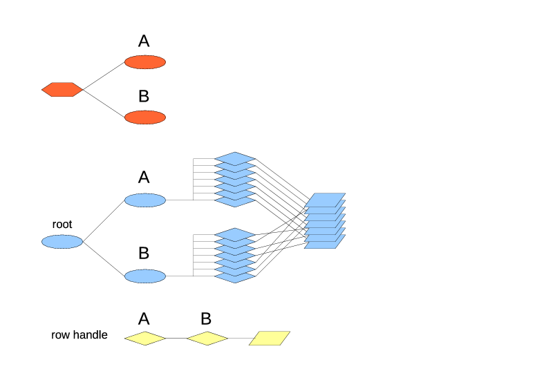
Continuing our excursion into the internals of the table, the next example is of two parallel leaf index types:

TableType
+-IndexType A
+-IndexType B

The resulting internal arrangement is shown on Fig. 8.

Fig. 8 Two top-level index types.

Each index type produces exactly one index under the root (since the top-level index types always produce one index). Both indexes contain the same number of rows, and exactly the same rows. When a row is added to the table, it's added to all the leaf index types (one actual index of each type). When a row is deleted from the table, it's deleted from all the leaf index types. So the total is always the same. However the order of rows in the indexes may differ. The drawing shows the row references stacked in the same order as the index A because the index A is of the first leaf index type, and as such is the default one for the iteration.

The row handle contains the iterators for both paths, A and B. It's pretty normal to find a row through one index type and then iterate from there using the other index type.

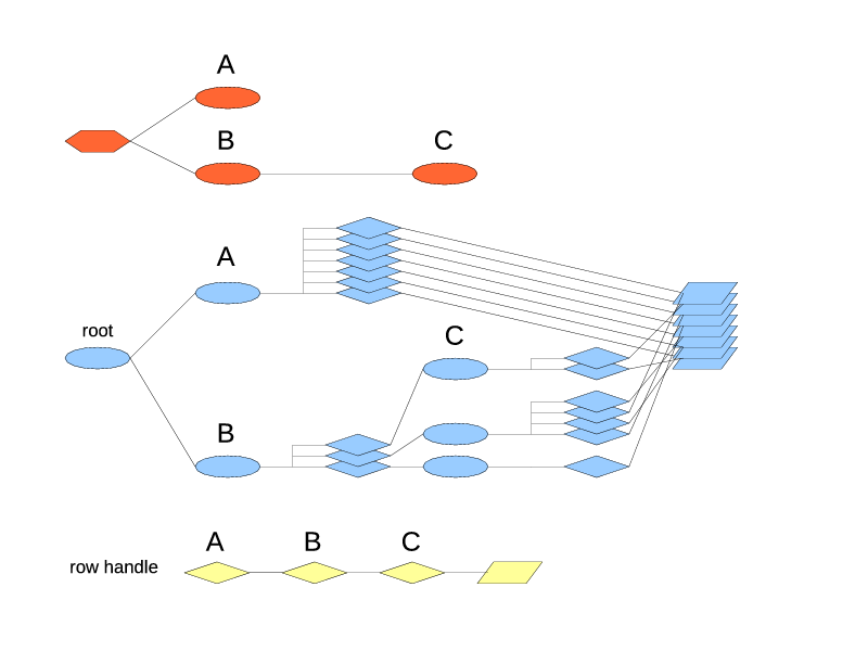
The next example on Fig. 9 has a "primary" index with a unique key and a "secondary" index that groups the records:

TableType
+-IndexType A
+-IndexType B
  +-IndexType C

Fig. 9. A "primary" and "secondary" index type.

The index type A still produces one index and references all the rows directly. The index of type B produces the groups, with each group getting an index of type C. The total set of rows referrable through A and through B is still the same but through B they are split into multiple groups.

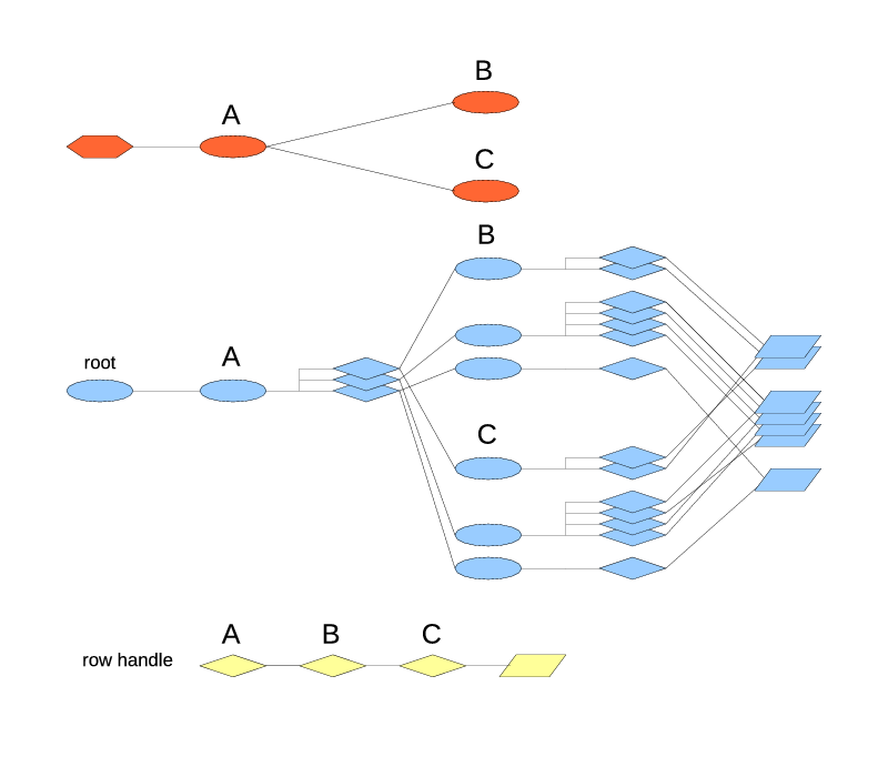
And Fig. 10 shows two leaf index types nested under one non-leaf.

TableType
+-IndexType A
  +-IndexType B
  +-IndexType C

Fig. 10. Two index types nested under one.

As usual, there is only one index of type A, and it splits the rows into groups. The new item in this picture is that each group has two indexes in it: one of type B and one of type C. Both indexes in the group contain the same rows. They don't decide, which rows they get. The index A decides, which rows go into which group. Then if the group 1 contains two rows, indexes B1 and C1, would both contain two rows each, the exact same set. The stack of row references has been visually split by groups to make this point more clear.

This happens to be a pretty useful arrangement: for example, B might be a hash index type, or in the future, a sorted index type, allowing to find the records by the key (and for the sorted index, to iterate in the order of keys), while C might be a FIFO index, keeping the insertion order, and maybe keeping the window size limited.

That's pretty much it for the basic index topologies. Some much more complex index trees can be created, but they would be the combinations of the examples shown. Also, don't forget that every extra index type adds overhead in both memory and CPU time, so avoid adding indexes that are not needed.

One more fine point has to do with the replacement policies. Consider that we have a table that contains the rows with the single field:

id int32

And the table type has two indexes:

TableType
+-IndexType "A" HashIndex key=(id)
+-IndexType "B" FifoIndex limit=3

Then we send there the rowops:

INSERT id=1
INSERT id=2
INSERT id=3
INSERT id=2

The second insert of id=2 triggers the replacement policy in both index types. In the index A it is a duplicate key and will cause the removal of the previous row with id=2. In the index B it overflows the limit and pushes out the oldest row, the one with id=1. If both records get deleted, the resulting table contents will be 2 rows (shown in FIFO order):

id=3
id=2

Which is probably not the best outcome. It might be tolerable with a FIFO index and a hashed index but gets even more annoying if there are two FIFO index types in the table: one top-level limiting the total number of rows, another one nested under a hashed index, limiting the number of rows per group, and they start conflicting this way with each other.

So the FIFO index is actually smart enough to avoid such problems: it looks at what the preceding indexes have decided to remove, checks if any of these rows belong to its group, and adjusts its calculation accordingly. In this example the index B will find out that the row with id=2 is already displaced by the index A. That leaves only 2 rows in the index B, so adding a new one will need no displacement. The resulting table contents will be

id=1
id=3
id=2

However here the order of index types is important. If the table were to be defined as

TableType
+-IndexType "B" FifoIndex limit=3
+-IndexType "A" HashIndex key=(id)

then the replacement policy of the index type B would run first, find that nothing has been displaced yet, and displace the row id=1. After that the replacement policy of the index type A will run, and being a hashed index, it doesn't have a choice, it has to replace the row id=2. And both rows end up displaced.

If the situations with automatic replacement of rows by the keyed indexes may arise, always make sure to put the keyed leaf index types before the FIFO leaf index types. However if you always diligently send a DELETE before the INSERT of the new version of the recond, then this problem won't occur and the order of index types will not matter.

The index tree, part 2

Let's use the Fig. 3 from the last post to go through how the other index-related operations work.

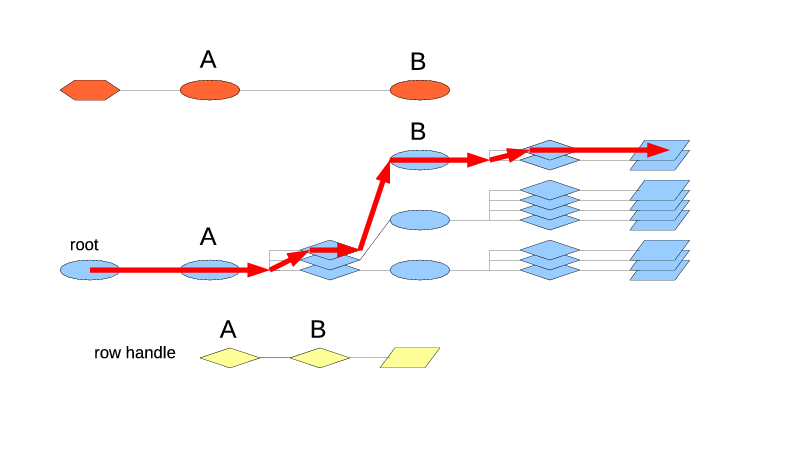
The iteration through the whole table starts with begin() or beginIdx(), the first being a form of the second that always uses the first leaf index type. BeginIdx() is fairly straightforward: it just follows the path from the root to the leaf, picking the first position in each index along the way, until it hits the RowHandle, as is shown in Fig. 4. That found RowHandle becomes its result. If the table is empty, it returns the NULL row handle.

If you specify a non-leaf index type as an argument of beginIdx(), the look-up can not just stop there because the non-leaf indexes are not directly connected to the row handles. It has to go through the whole chain to a leaf index. So, for a non-leaf index type argument the look-up is silently extended to its first leaf index type.

Fig. 4. Begin(), beginIdx($itA) and beginIdx($itB) work the same for this table.

The next pair is find() and findIdx(). As usual, find() is the same thing as findIdx() on the table's first leaf index type. It also follows the path from the root to the target index type. On each step it tries to find a matching position in the current index. If the position could not be found, the search fails and a NULL row handle is returned. If found, it is used to progress to the next index.

As has been mentioned before, the search always works internally on a RowHandle argument. If a plain Row is used as an argument, a new temporary RowHandle will be created for it, searched, and then freed after the search. This works well for two reasons. First, the indexes already have the functions for comparing two row handles to build their ordering. The same functions are reused for the search. Second, the row handles contain not only the index iterators but also the cached information from the rows, to make the comparisons faster. The exact kind of cached information varies by the index type. The FIFO indexes use none. The hashed indexes calculate a hash of the key field values, that will be used as a quick differentiator for the search. This information gets created when the row handle gets created. Whether the row handle is then used to insert into the table or to search in it, it's then used in the same way, to speed up the comparisons.

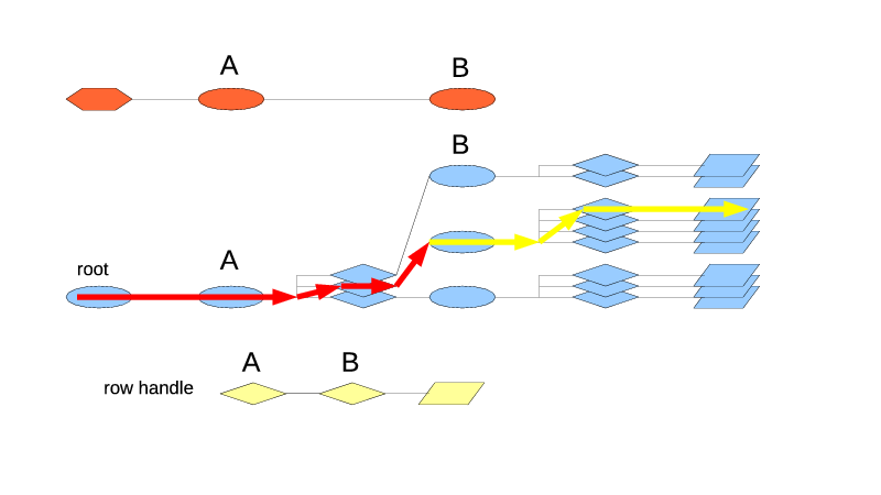
For findIdx(), the non-leaf index type arguments behave differently than the leaf ones: up to and including the index of the target type, the search works as usual. But then at the next level the logic switches to the same as in beginIdx(), going for the first row handle of the first leaf sub-index. This lets you find the first row handle of the matching group under the target index type.

If you use $table->findIdx($itA, $rh), on Fig. 5 it will go through the root index to the index A. There it will try to find the matching position. If none is found, the search ends and returns a NULL row handle. If the position is found, the search progresses towards the first leaf sub-index type. Which is the index type B, and which conveniently sits in this case right under A. The position in the index A determines, which index of type B will be used for the next step. Suppose it's the second position, so the second index of type B is used. Since we're now past the target index A, the logic used is the same as for beginIdx(), and the first position in B2 is picked. Which then leads to the first row handle of the second sub-stack of handles.

Fig. 5 FindIdx($itA, $rh) goes through A and then switches to the begin() logic.

The method firstOfGroupIdx() allows to navigate within a group, to jump from some row somewhere in the group to the first one, and then from there iterate through the group. The example of manual aggregation made use of it.

The Fig. 6 shows the example of $table->firstOfGroupIdx($itB, $rh), where $rh is pointing to the third record in B2. What it needs to do is go back to B2, and then execute the begin() logic from there on. However, remember, the row handle does not have a pointer to the indexes in the path, it only has the iterators. So, to find B2, the method does not really back up from the original row. It has to start back from the root and follow the path to B2 using the iterators in $rh. Since it uses the ready iterators, this works fast and requires no row comparisons. Once B2 (an index of type B) is reached, it goes for the first row in there.

FirstOfGroupIdx() works on both leaf and non-leaf index type arguments in the same way: it backs up from the reference row to the index of that type and executes the begin() logic from there. Obviously, if you use it on a non-leaf index type, the begin()-like part will follow its first leaf index type.

Fig. 6. FirstOfGroupIdx($itB, $rh)

The method nextGroupIdx() jumps to the first row of the next group, according to the argument index type. To do that, it has to retrace one level higher than firstOfGroupIdx(). Fig. 7 shows that $table->nextGroupIdx($itB, $rh) that starts from the same row handle as Fig. 6, has to logically back up to the index A, go to the next iterator there, and then follow to the first row of B3.

As usual, in reality there is no backing up, just the path is retraced from the root using the iterators in the row handle. Once the parent of index type B is reached (which is the index of type A), the path follows not the iterator from the row handle but the next one (yes, copied from the row handle, increased, followed). This gives the index of type B that contains the next group. And from there the same begin()-like logic finds its first row.

Same as firstOfGroupIdx(), nextGroupIdx() may be used on both the leaf and non-leaf indexes, with the same logic.

Fig. 7. NextGroupIdx($itB, $rh)

It's kind of annoying that firstOfGroupIdx() and nextGroupIdx() take the index type inside the group while findIdx() uses takes the parent index type to act on the same group. But as you can see, each of them follows its own internal logic, and I'm not sure if they can be reconciled to be more consistent.

At the moment the only navigation is forward. There is no matching last(), prev() or lastGroupIdx() or prevGroupIdx(). They are in the plan, but so far they are the victims of corner-cutting.

The index tree, part 1

The index types in a table type can form a pretty much arbitrary tree. Following the common tree terminology, the index types that have no other index types nested in them, are called the leaf index types. Since there seems to be no good one-word naming for the index types that have more index types nested in them ("inner"? "nested" is too  confusing), I simply call them non-leaf.

At the moment the Hashed index types can be used only in both leaf and non-leaf positions. The FIFO index types must always be in the leaf position, they don't allow the further nesting.

Now is the moment to look deeper into what is going on inside a table. Note that I've been very carefully talking about "index types" and not "indexes". In this post the difference matters. The index types are in the table type, the indexes are in the table. One index type may generate multiple indexes.

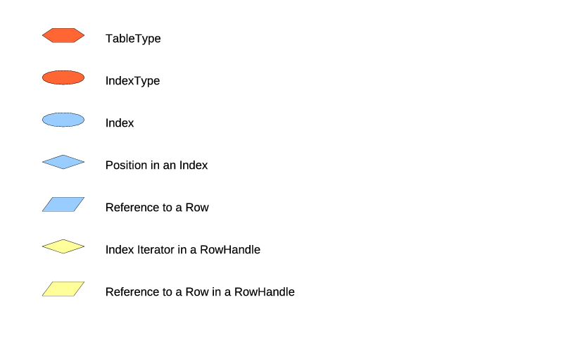
This will become clearer after you see the illustrations. I really hate doing the drawings, but here they are really necessary for the understanding, and way too complex for the ASCII-art. But first, the legend on Fig. 1.

Fig. 1. Drawings legend.

The nodes belonging to the table type are shown in red, the nodes belonging in the table are shown in blue, and the contents of the RowHandle is shown separately in yellow. The lines on the drawings represent not exactly pointers as such but more of the logical connections that may be more complicated than the simple pointers.

The lines in the RowHandle don't mean anything at all, they just show that the parts go together. In reality a RowHandle is a chunk of memory, with various elements placed in that memory. As far as indexes are concerned, the RowHandle contains an iterator for every index where it belongs. This lets it know its position in the table, to iterate along every index, and, most importantly, to be removed quickly from every index. A RowHandle belongs to one index of each index type, and contains the matching number of iterators in it.

The table type is shown as a normal flat tree. But the table itself is more complex and becomes 3-dimensional. Its "view from above" matches the table type's tree but the data grows "up" in the third dimension.

Let's start with the simplest case: a table type with only one index type. Whether the index type is hash or FIFO, doesn't matter here.

TableType
+-IndexType "A"

Fig. 2 shows the table structure.

Fig. 2. One index type.

The table here always contains exactly one index, matching the one defined index type, and the root index. The root index is very dumb, its only purpose is to tie together the multiple top-level indexes into a tree.

The only index of type A provides an ordering of the records, and this ordering is used for the iteration on the table.

For the next example let's look at the straight nesting at fig. 3.

TableType
+-IndexType "A"
  +-IndexType "B"

Fig. 3. Straight nesting.

The stack of row references is shown visually divided to match the indexing, but in reality there is no special division. This was done purely to make the picture easier to read.

There is still only one index of type A. And this is always the case with the top-level indexes, there is only one of them. This index divides the rows into 3 groups. Just like the rows in a leaf index, the groups in a non-leaf index are ordered in some way.

Each group then has its own second-level index of type B. Which then defines an order for the rows in it. To reiterate: the index of type A splits the rows by groups, then the group's index of type B defines the order of the rows in the group.

So what happens when we iterate through the table and ask for the next row handle? The current row handle contains the iterators in the indexes of types A and B. The easy thing is to advance the iterator of type B. Yeah, but in which index? The figure shows 3 indexes of type B, let's call them B1, B2 and B3. The iterator of type B in the row handle tells the relative position in the index, but it doesn't tell, which index it is. We need to step back and look at the index type A. It's the top-level index type, so there is always only one index for it. Then we take the iterator of type A and find this row's group in the index A. The group contains the index of type B, say B1. We can then take this index B1, take the iterator of type B from the row handle, and advance this iterator in this index. If the advance succeeded, then great, we've got the next row handle. But if the current row was the last row in B1, we need to step back to the index A again, advance the current row handle's iterator of type A there, find its index B2, and pick the first row handle of B2.

This process is what happens when we say $table->nextIdx($itB, $rh) or equivalently $rh->nextIdx($itB). The iteration goes by the leaf index type B, however it relies on all the index types in the path from the table type to B. If we do $rh->next(), the result is the same because the first leaf index type is used as the default index type for the iteration.

If we do $rh->next($itA),  the semantics is still the same: return the next row handle (not the next group). There is no way to get to the row handle without going all the way through a leaf index. So when a non-leaf index type is used for the iteration, it gets implicitly extended to its first nested leaf index type.

What would happen if a new row gets inserted, and the index type A determines that it does not belong to any of the existing groups? A new group will be created and inserted in the appropriate position in A's order. This group will have a new index of type B created, and the new row inserted in that index.

What would happen if both rows in B1 are removed? B1 will become empty and will be collapsed. The index A will delete the B1's group and B1 itself, and will remain with only two groups. The effect propagates upwards: if all the rows are removed, the last index of type B will collapse, then the index A will become empty and also collapse and be deleted. The only thing left will be the root index that stays in the existence no matter what.

When a table is first created, it has only the root index. The rest of the indexes pop into the existence as the rows get inserted. If you wonder, yes, this does apply to a table type with only one index type as well. Just this point has not been brought up until now.

Among all this froth of creation and collapse the iterators stay stable. Once a row is inserted, the indexes leading to it are not going anywhere (at least until that row gets removed). But since other rows and groups may be inserted around it, the notion of what row is next, will change over time.

memory management

The memory is managed in Triceps using the reference counters. Each Triceps object has a reference counter in it. There is an Autoref template that produces reference objects. As the references are copied around between these objects, the reference counts in the target objects are adjusted. When the reference count drops to 0, the target object gets destroyed. While there are live references, the object can't get destroyed from under them. All nice and well and simple, however still possible to get wrong.

The major problem with the reference counters is the reference loops. If object A has a reference to object B, and object B has a reference (possibly, indirect) to object A, then neither of them will ever be destroyed. Many of these cases can be resolved by keeping a reference in one direction and a plain pointer in the other.  This of course introduces the problem of hanging pointers, so extra care has to be taken to not reference them. There also are the unpleasant situations when there is absolutely no way around the reference loops. For example, the Triceps label's method may keep a reference to the next label, where to send its processed results. If the labels are connected into a loop (a perfectly normal occurrence), this would cause a reference loop. Here the way around is to know when all the labels are no longer used (before the thread exit), and explicitly tell them to clear their references to the other labels. This breaks up the loop, and then bits and pieces can be collected by the reference count logic.

The reference counting maybe single-threaded or multi-threaded. If an object may only be used inside one thread, the references to it use the faster single-threaded counting.In C++ it's real important to not access and not reference the single-threaded objects from multiple threads. In Perl, when a new thread is created, only the multithreaded objects from the parent thread become accessible to it, the rest become undefined, so the issue gets handled automatically (as of version 1.0 even the potentially multithreaded objects are still exported to Perl as single-threaded, with no connection between threads yet).

The C++ objects are exported into Perl through wrappers. The wrappers perform the adaptation between Perl reference counting and Triceps reference counting, and sometimes more helper functions. Perl sees them as blessed objects, from which you can inherit and otherwise treat like normal objects.

When the Perl references are copied between the variables, this increases the Perl reference count to the same wrapper object. However if an object goes into the C++ land, and then is extracted back (such as, create a Rowop from a Row, and then extract the Row from that Rowop), a brand new wrapper gets created. It's the same underlying C++ object but with multiple wrappers. You can't tell that it's the same object by comparing the Perl references, because they may be pointing to the different wrappers. However Triceps provides the method same() that compares the data inside the wrappers. It can be used as

$row1->same($row2)

and if it returns true, then both $row1 and $row2 point to the same underlying row. Note also that if you inherit from the Triceps objects and add some extra data to them, none of that data nor even your derived class identity will be preserved when a anew wrapper is created from the underlying C++ object.

API introduction

As mentioned before, at the moment Triceps provides the APIs in C++ and Perl. They are similar but not quite the same, because the nature of the compiled and scripted languages is different. The C++ API is more direct and expects discipline from the programmer: if some incorrect arguments are passed, everything might crash. The Perl API should never crash. It should detect any incorrect use and report an orderly error. Besides, the idioms of the scripted languages are different from the compiled languages, and different usages become convenient.


The Perl API is implemented in XS. Some people, may wonder, why not SWIG? SWIG would automatically export the API into many languages, not just Perl. The problem with SWIG is that it just maps the API one to one.  And this doesn't work any good, it makes some very ugly APIs with abilities to crash. Which then have to be wrapped into more scripting code before they become usable. So then why bother with SWIG, easier to just use the scripting language's native extension methods. Another benefit of the native support is the access to the correct memory management.

In general, I've tried to avoid the premature optimization. The idea is to get it working at all first, and then bother about working fast. Except for the cases when the need for optimization looked obvious, and the logic intertwined with the general design strongly ehough, that if done one way, would be difficult to change in the future. We'll see, if these "obvious" cases really turn out to be the obvious wins, or will they become a premature-optimization mess.

Going forward, I'll try to split the subjects into the separate posts, centered around Perl API, C++ API, or guts of the (C++) implementation and tag them as such. Feel free to pick only the ones you're interested in.Some of the posts still will be general, and have all three tags.